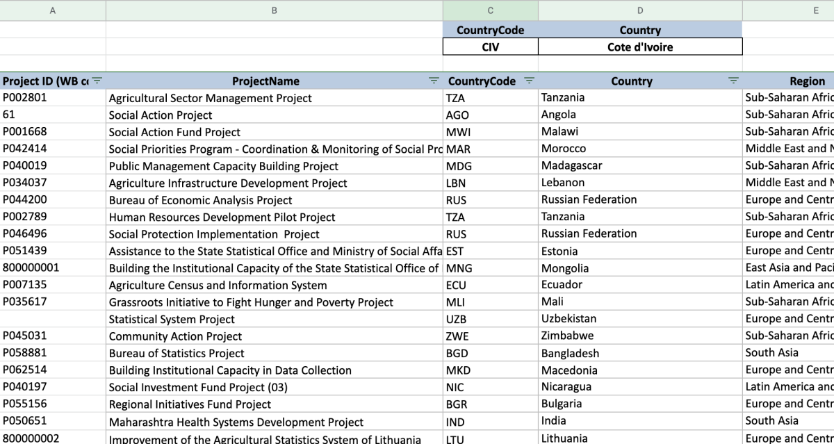
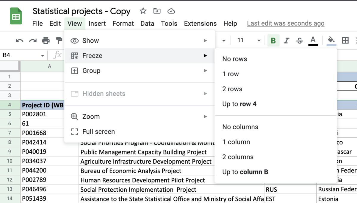
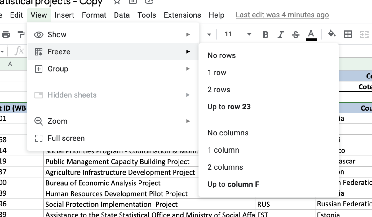
The fix for this situation is to freeze columns and rows. Freezing them will allow you to move as far down and to the right, as you want so your column and row labels don’t leave your sight. In the Google Sheet example below, I would like to freeze the first two columns and the first three rows to make identifying cells easier in my document. To start the freezing process, I first on the view tab and freeze option shown in the illustration below. There are six different options for freezing listed below.
1 row 2 rows up to 4 rows (Varies depending on the cell selected) 1 column 2 columns up to 8 columns (Varies depending on the cell selected)
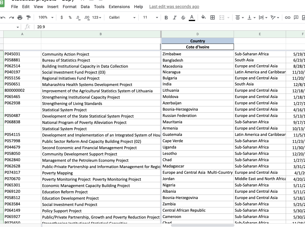
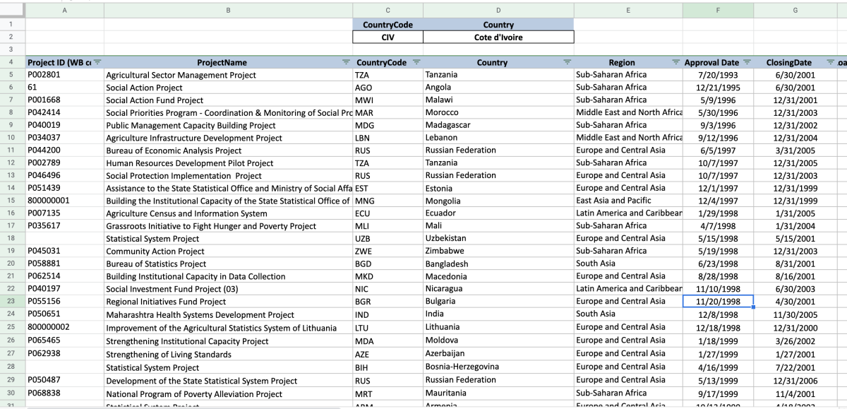
For my situation, I chose the option to have two columns freeze. I had to go back into the view tab to choose the two-row freeze option. You can tell where the columns and rows are frozen by the thick gray dividing line. Note that the third option for columns and rows is not fixed. Moving your cursor to the coordinate where the freeze needs to start will change those options. In the illustration below, the freeze was removed by choosing the no rows and no columns options. Notice that cell F23 was chosen. Because F23 was chosen, the third option changed to allow freezes for all columns to the left of column F and all rows at and above row 23. This content is accurate and true to the best of the author’s knowledge and is not meant to substitute for formal and individualized advice from a qualified professional. © 2022 Joshua Crowder